Model explainer — theory, significance, and formulas.

An algorithm that sidesteps the biggest weakness of Markowitz optimization — the inverse of the covariance matrix — by first grouping assets into "clusters of things that move alike" and then splitting risk among those clusters.

Anyone who actually runs Markowitz optimization soon notices that the results get strange as the number of holdings grows: 99% on one name and 0.1% on another, or completely different weights when the inputs are perturbed by even a tiny amount.

The root cause is the "inverse of the covariance matrix (Σ⁻¹)" inside the Markowitz formula. When the number of holdings is large relative to the data length, that inverse becomes numerically unstable, and the instability propagates directly into the weights.

In 2016, López de Prado started from the question "what if we just don't invert the matrix at all?" and borrowed clustering techniques from machine learning to propose HRP.

HRP computes weights in three steps — let's walk through each with diagrams.

① Tree Clustering — bundling similar assets into a tree

First, all pairwise correlations (ρ) are converted into distances: d(i, j) = √(½ · (1 − ρᵢⱼ)). A correlation near 1 yields a distance near 0; a negative correlation produces a larger distance. The closest pair of assets is merged first, then the next-closest, and so on, building a tree structure (dendrogram). As shown below, "assets that move alike" naturally fall on the same branch, and "assets that move differently (e.g., a bond ETF like TLT)" join the tree last.

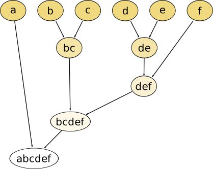
The figure above shows the "general shape" of a dendrogram — close points pair up first, then progressively more distant groups merge, until all data is bound into one tree. As the dashed line illustrates, the number of clusters depends on where you cut. HRP uses this tree directly as the "asset cluster structure." The next figure shows the dendrogram this tool actually produces for a 6-holding example.

② Quasi-Diagonalization — reordering the covariance matrix

The rows and columns of the covariance matrix are reordered using the "similar-assets adjacent" ordering from the dendrogram. The originally scattered values become concentrated along the diagonal — hence "quasi-diagonal". This ordering is the setup for the next step's recursive bisection.

③ Recursive Bisection — split groups in two and allocate weights

Split the ordered list of assets in two. Compute each half's "cluster variance," and assign a smaller weight to the higher-variance half and a larger weight to the lower-variance half (inverse-variance allocation). Then split each half again and repeat recursively all the way down to individual assets. By the end, every asset has a weight.

The key point is that, unlike Markowitz, HRP never inverts the full covariance matrix Σ⁻¹. At each step you only compare "the variance of two halves," so even when the number of assets is large and the data window is short — conditions that make Σ numerically unstable — the result does not blow up. This is the core of HRP's robustness.

• Gives more stable weights than Markowitz when the asset count is high and the data window is short
• Designed so that a blow-up in one asset is contained within its cluster
• Used in practice for weight selection in risk-parity ETFs and multi-asset funds
• Especially well-suited to asset classes with short histories — crypto, newly launched ETFs, etc.

HRP focuses on robust diversification rather than aggressively chasing expected return — it does not reach the "point on the efficient frontier" that Markowitz can offer in theory. The cluster results are also only meaningful if the correlation structure across assets stays reasonably stable over time.

• SSRN — Marcos M. López de Prado author page · The HRP preprint and follow-up research, posted directly by the author
• Wikipedia — Hierarchical Clustering · Overview of tree clustering, linkage methods and dendrograms
• Wikipedia — Risk Parity · The general concept of risk parity and where HRP fits in